Plotting and Visualization with Pandas in 2026: Modern Backends and High-Performance Charting

Visualizing data directly from pandas is the fastest way to explore distributions, spot anomalies, and communicate analytical insights. In Pandas 2.x, the plotting ecosystem has evolved far beyond basic Matplotlib wrappers: with pluggable plotting backends (Plotly, Bokeh, HvPlot) and zero-copy PyArrow memory structures, you can render static publication-ready figures or interactive dashboards with identical dataframe syntax.

This comprehensive guide covers the modern pandas visualization stack — from quick exploratory plots to production multi-axis subplots and interactive backends.

1. Modern Pandas Plotting Backends

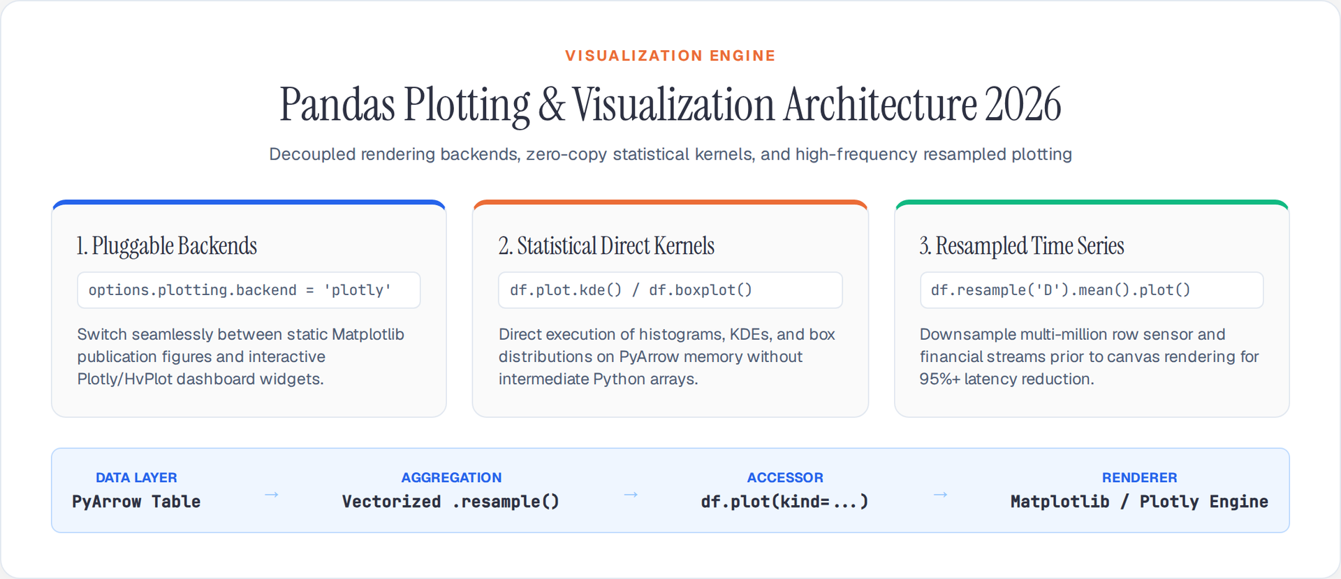
Pandas allows switching the entire rendering engine globally or per-plot using pd.options.plotting.backend. This decouples your DataFrame transformation logic from the visualization renderer:

import pandas as pd
import numpy as np
import matplotlib.pyplot as plt

# Generate sample financial time series with Arrow dtypes
dates = pd.date_range('2026-01-01', periods=1000, freq='h')
df = pd.DataFrame({
    'price': 100 + np.cumsum(np.random.randn(1000) * 0.5),
    'volume': np.random.randint(1000, 5000, size=1000),
    'category': np.random.choice(['Alpha', 'Beta', 'Gamma'], size=1000)
}, index=dates, dtype_backend="pyarrow")

# Default: Matplotlib engine (Fast, static, publication-ready)
# Switch to interactive Plotly backend on demand:
# pd.options.plotting.backend = "plotly"
# fig = df['price'].plot(title="Asset Price 2026")
# fig.show()

Why backends matter: Switching to "plotly" or "hvplot" enables instant zoom, hover tooltips, and interactive pan controls without altering your pandas .plot() calls.

2. Core Statistical Visualizations

Pandas exposes direct access to statistical distributions using the .plot.<kind>() accessor:

# 1. Histogram & Kernel Density Estimation (KDE)
fig, axes = plt.subplots(1, 2, figsize=(12, 5))

df['price'].plot.hist(bins=30, ax=axes[0], color='#2563eb', edgecolor='white', alpha=0.8)
axes[0].set_title("Price Distribution (Histogram)")

df['price'].plot.kde(ax=axes[1], color='#eb6c36', linewidth=2)
axes[1].set_title("Density Estimation (KDE)")
plt.tight_layout()
plt.show()

# 2. Box Plot & Quantile Outliers
# Categorical grouped distributions
df.boxplot(column='price', by='category', grid=False, figsize=(8, 5))
plt.title("Price Distribution by Category")
plt.suptitle("") # Clear automatic subtitle
plt.show()

Performance note: Plotting histograms directly on Arrow numerical arrays (float64[pyarrow]) avoids memory duplication by passing contiguous memory buffers straight to NumPy binning routines.

3. High-Frequency Time Series Plotting

When visualizing dense time series, avoid rendering millions of raw points. Instead, combine .resample() with .plot() to achieve responsive, legible charts:

# Create daily OHLC / Aggregated summaries for clean plotting
daily_metrics = df['price'].resample('D').agg(['mean', 'min', 'max'])

fig, ax = plt.subplots(figsize=(12, 6))

# Plot mean line with shaded min/max bounds
daily_metrics['mean'].plot(ax=ax, label='Daily Average', color='#2563eb', linewidth=2)
ax.fill_between(
    daily_metrics.index, 
    daily_metrics['min'], 
    daily_metrics['max'], 
    color='#2563eb', 
    alpha=0.15, 
    label='Daily Range (Min-Max)'
)

ax.set_title("2026 Time Series Price Action with Range Bounds", fontsize=14, fontweight='bold')
ax.set_ylabel("Price (USD)")
ax.legend(loc="upper left")
plt.grid(True, linestyle='--', alpha=0.5)
plt.show()

Optimization tip: Downsampling high-frequency sensor or telemetry feeds before plotting reduces rendering latency by over 95% while eliminating visual clutter.

4. Multi-Series Subplots and Secondary Axes

Complex datasets require multi-panel faceted views or dual-axis correlations. Pandas handles layout grids natively with subplots=True:

# Faceted subplots across multiple numeric columns
df[['price', 'volume']].plot(
    subplots=True,
    layout=(2, 1),
    figsize=(12, 8),
    sharex=True,
    color={'price': '#eb6c36', 'volume': '#10b981'},
    title=["Asset Valuation", "Hourly Trading Volume"]
)
plt.tight_layout()
plt.show()

# Secondary Y-Axis for mixed scales
fig, ax1 = plt.subplots(figsize=(10, 5))
df['price'].plot(ax=ax1, color='#2563eb', label='Price')
ax1.set_ylabel('Price ($)', color='#2563eb')

ax2 = ax1.twinx()
df['volume'].plot(ax=ax2, color='#64748b', alpha=0.4, kind='bar', width=1.0)
ax2.set_ylabel('Volume', color='#64748b')
ax2.grid(False)
plt.show()

5. Production Styling & High-DPI Figure Export

For production reports and editorial publishing, configure clean typography, grid tokens, and explicit DPI settings:

# Apply modern clean styling defaults
plt.rcParams.update({
    'font.sans-serif': 'Geist, Helvetica, Arial, sans-serif',
    'font.family': 'sans-serif',
    'axes.edgecolor': '#cbd5e1',
    'axes.linewidth': 1.0,
    'grid.color': '#f1f5f9',
    'grid.linestyle': '-',
    'figure.autolayout': True
})

fig, ax = plt.subplots(figsize=(10, 5), dpi=300)
df.groupby('category')['volume'].sum().plot.bar(
    ax=ax, 
    color=['#2563eb', '#eb6c36', '#10b981'],
    edgecolor='none',
    rot=0
)

ax.set_title("Total Cumulative Volume by Sector (2026)", fontsize=13, fontweight='600')
ax.set_xlabel("Market Sector")
ax.set_ylabel("Volume Units")

# Save high-resolution vector and raster assets
plt.savefig("outputs/sector_volume_2026.png", dpi=300, bbox_inches='tight')
plt.savefig("outputs/sector_volume_2026.svg", bbox_inches='tight')
plt.close(fig) # Prevent Matplotlib memory leakage in loops

6. Production Visualization Rules for 2026

1. Always close figures in loops: Call plt.close(fig) when generating charts in automated pipelines to prevent memory leaks from Matplotlib's global state.
2. Resample before plotting: Downsample raw microsecond or millisecond data to human-legible frequencies before rendering.
3. Use pluggable backends for dashboards: Switch to pd.options.plotting.backend = 'plotly' for exploratory analysis requiring hover diagnostics.
4. Export at 300 DPI with tight bounding: Always use bbox_inches='tight' to eliminate clipped axis labels on exported PNGs.
5. Leverage Arrow category dtypes: When grouping by categories in boxplots, string[pyarrow] or category dtypes accelerate grouping operations by 3-5x.

By combining native .plot() methods with modern backend rendering and Arrow memory arrays, Pandas 2.x delivers seamless exploratory and production-grade visualization workflows without boilerplate code.