Mastering Data Structures with Pandas: A Comprehensive Guide (2026)

Pandas is the foundation of data manipulation in Python, but understanding its core data structures at an architectural level is what separates slow, memory-hungry scripts from high-performance production pipelines.

In modern Pandas (2.x and beyond), data structures have evolved significantly with PyArrow backends, nullable data types, and copy-on-write optimizations. This guide breaks down the core Pandas data structures—Series, DataFrame, and Index—how they operate under the hood, and how to write idiomatic, memory-efficient code.

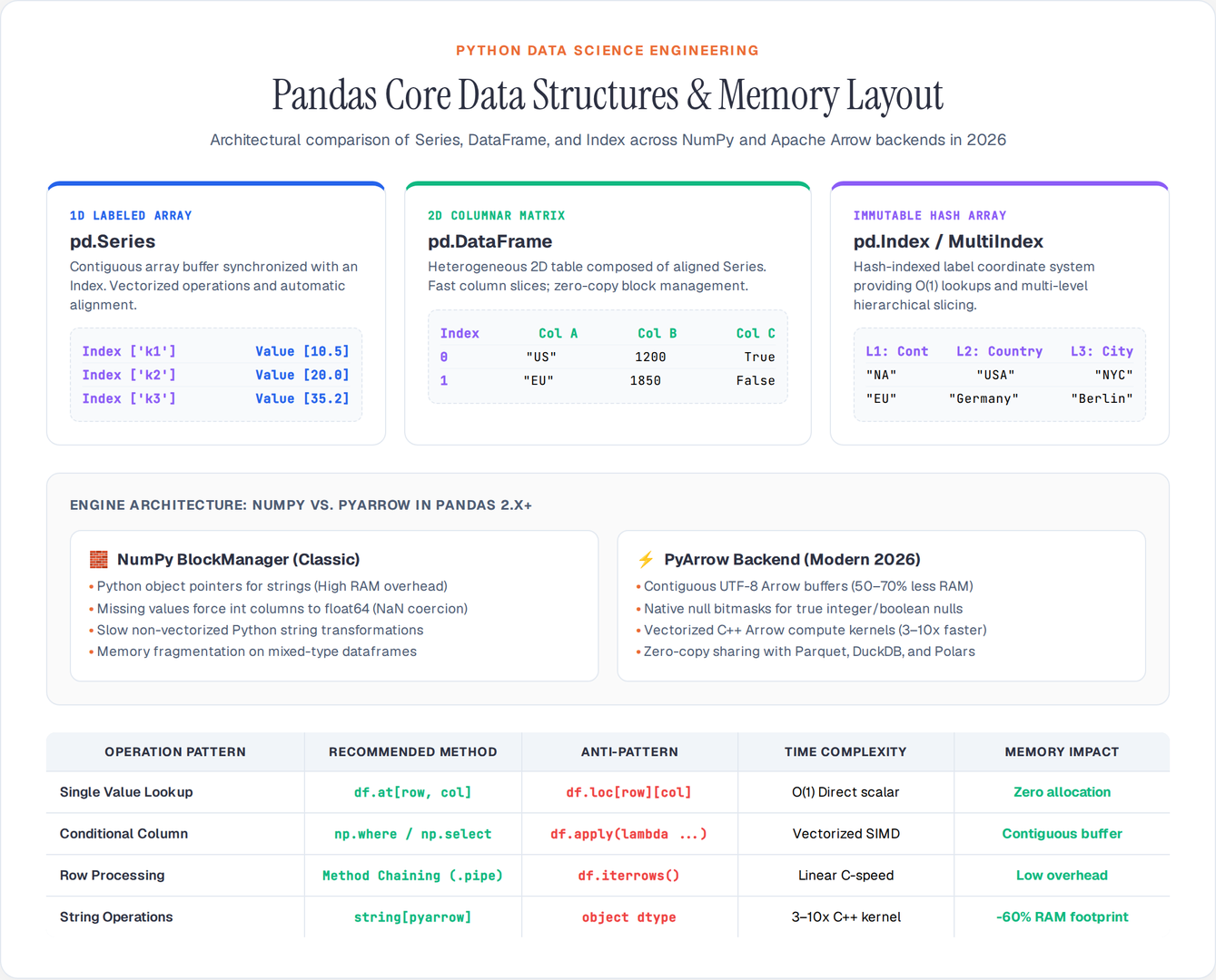
1. The Core Pandas Architecture: Series, DataFrame, and Index

At its core, Pandas coordinates three primary data structures:

• pd.Series: A 1D labeled array capable of holding any data type. Conceptually a single column with an explicit index.
• pd.DataFrame: A 2D labeled tabular structure composed of aligned Series sharing a common row index.
• pd.Index: An immutable, hash-backed array that provides fast label lookups and automatic alignment for Series and DataFrames.

import pandas as pd
import numpy as np

# A Series is an indexed 1D array
s = pd.Series([10.5, 20.0, 35.2], index=["cpu_1", "cpu_2", "cpu_3"], name="usage_pct")

# A DataFrame aligns multiple Series along a shared Index
df = pd.DataFrame({
    "usage_pct": s,
    "cores": [4, 8, 16],
    "region": ["us-east", "us-west", "eu-central"]
}, index=["cpu_1", "cpu_2", "cpu_3"])

print(df)

Memory Layout: Columnar Storage vs. Row-Oriented Records

Under the hood, a DataFrame is columnar, not row-oriented. Each column is stored as a contiguous memory buffer (either a NumPy array or an Apache Arrow chunked array).

This columnar layout has massive performance implications:

• Extracting or transforming an entire column is extremely fast (zero-copy slice or contiguous memory vectorization).
• Iterating row-by-row (for row in df.iterrows()) is orders of magnitude slower because Pandas must reconstruct a Series object for every single row on the fly.

2. Deep Dive: pd.Series (1D Labeled Array)

A Series consists of two synchronized components: the values array and the index label array.

import pandas as pd

# Creating a Series with explicit dtype and index
prices = pd.Series(
    data=[49.99, 129.50, 19.99, 89.00],
    index=["sku_101", "sku_102", "sku_103", "sku_104"],
    dtype="float64",
    name="price_usd"
)

# Inspecting internal attributes
print(f"Values array: {prices.values}")       # Underlying array buffer
print(f"Index labels: {prices.index}")         # Index object
print(f"Memory bytes: {prices.memory_usage(deep=True)}")

Fast Label vs. Positional Access

Pandas provides distinct indexers to prevent ambiguity between integer positions and integer labels:

• .loc[]: Label-based indexing (inclusive of stop boundary).
• .iloc[]: Integer position-based indexing (exclusive of stop boundary, standard Python slicing).
• .at[] / .iat[]: Scalar-optimized accessors (up to 5x faster than .loc/.iloc for single-value lookups in loops).

# Label access
print(prices.loc["sku_102"])  # 129.50

# Position access
print(prices.iloc[1])         # 129.50

# Slicing with labels (inclusive)
print(prices.loc["sku_101":"sku_103"])

# Fast scalar retrieval
print(prices.at["sku_102"])   # Scalar lookup

Vectorized Arithmetic and Automatic Label Alignment

Operations between Series automatically align on index labels, not array positions. If labels do not match, Pandas inserts NaN (or null in Arrow):

s1 = pd.Series([10, 20, 30], index=["a", "b", "c"])
s2 = pd.Series([5, 15, 25], index=["b", "c", "d"])

# Automatic alignment
total = s1 + s2
print(total)
# Output:
# a     NaN
# b    25.0
# c    45.0
# d     NaN
# dtype: float64

3. Deep Dive: pd.DataFrame (2D Tabular Structure)

A DataFrame combines multiple Series into a two-dimensional tabular matrix with row labels (df.index) and column labels (df.columns).

import pandas as pd
import numpy as np

# Constructing DataFrame from records or dictionary of arrays
data = {
    "device_id": ["dev_01", "dev_02", "dev_03", "dev_04"],
    "battery_pct": [98.5, 45.0, 12.2, 87.0],
    "status": ["active", "active", "warning", "active"],
    "readings_count": [1420, 890, 310, 2050]
}

df = pd.DataFrame(data).set_index("device_id")

Method Chaining with Modern Pandas

Modern idiomatic Pandas avoids in-place mutations (inplace=True is deprecated/discouraged across modern codebases). Instead, use method chaining with .assign(), .query(), and .pipe():

# Clean, readable, pipeline-driven transformation
processed_df = (
    df
    .query("battery_pct < 50.0")
    .assign(
        critical_flag=lambda x: x["battery_pct"] < 20.0,
        battery_ratio=lambda x: x["battery_pct"] / 100.0
    )
    .sort_values(by="battery_pct", ascending=True)
)

print(processed_df)

4. Understanding the Index and MultiIndex

The Index is the backbone of search and relational joins in Pandas. An Index is an immutable, hash-indexed structure enabling $O(1)$ scalar lookups.

MultiIndex (Hierarchical Indexing)

A MultiIndex allows you to represent higher-dimensional data (3D, 4D) in a standard 2D DataFrame:

# Creating a MultiIndex DataFrame
tuples = [
    ("North America", "USA", "New York"),
    ("North America", "USA", "San Francisco"),
    ("North America", "Canada", "Toronto"),
    ("Europe", "Germany", "Berlin"),
    ("Europe", "UK", "London")
]

index = pd.MultiIndex.from_tuples(tuples, names=["Continent", "Country", "City"])

sales_df = pd.DataFrame(
    data={"revenue_k": [1200, 1850, 920, 1100, 1400], "headcount": [45, 80, 30, 42, 60]},
    index=index
)

print(sales_df)

# Slicing at multiple levels using Cross-Section (xs)
usa_data = sales_df.xs("USA", level="Country")
print(usa_data)

5. Modern Data Types: NumPy vs. PyArrow Backend

In Pandas 2.x+, you can choose between classic NumPy storage backends and the high-performance Apache Arrow backend (dtype_backend="pyarrow").

Feature	Classic NumPy Backend	PyArrow Backend (dtype_backend="pyarrow")
String Storage	Python object pointers (high RAM overhead)	Contiguous UTF-8 Arrow string arrays
Missing Values	np.nan (forces integer columns to float)	Native null bitmask (true integer/boolean nulls)
Memory Consumption	Baseline (1.0x)	Up to 50–70% less RAM for string/mixed datasets
String Operations	Slow Python interpreter overhead	Vectorized C++ Arrow compute kernels (3–10x faster)
Interoperability	Requires copying data to Parquet/Polars	Zero-copy memory sharing via Arrow C Data Interface

Benchmarking PyArrow Strings in Action

import pandas as pd
import time

# Create 1,000,000 strings
raw_strings = [f"user_{i}@enterprise-domain-{i%50}.com" for i in range(1_000_000)]

# Standard NumPy/Object Series
s_numpy = pd.Series(raw_strings)

# PyArrow String Series
s_arrow = pd.Series(raw_strings, dtype="string[pyarrow]")

print(f"NumPy Object RAM : {s_numpy.memory_usage(deep=True) / 1024**2:.2f} MB")
print(f"PyArrow String RAM: {s_arrow.memory_usage(deep=True) / 1024**2:.2f} MB")

# Speed test on string transformation
t0 = time.perf_counter()
res_np = s_numpy.str.upper().str.contains("ENTERPRISE")
t_np = time.perf_counter() - t0

t0 = time.perf_counter()
res_arrow = s_arrow.str.upper().str.contains("ENTERPRISE")
t_arrow = time.perf_counter() - t0

print(f"NumPy string processing: {t_np:.3f}s")
print(f"PyArrow processing     : {t_arrow:.3f}s ({t_np / t_arrow:.1f}x speedup)")

6. Performance & Memory Optimization Rules

To get peak performance out of Pandas data structures:

1. Never Use Iterative Loops (for / iterrows)

Instead of df.iterrows(), use vectorized operations, .map(), or NumPy arrays:

# Anti-pattern: Slow iteration
# for idx, row in df.iterrows(): ...

# Best Practice: Vectorized condition with numpy select or np.where
df["category"] = np.where(df["battery_pct"] > 80, "High", "Low")

2. Downcast Numeric Types & Use Categoricals

Downcasting 64-bit numeric columns and converting low-cardinality strings to category dtypes slashes memory:

def optimize_dtypes(df: pd.DataFrame) -> pd.DataFrame:
    for col in df.columns:
        if df[col].dtype == "int64":
            df[col] = pd.to_numeric(df[col], downcast="integer")
        elif df[col].dtype == "float64":
            df[col] = pd.to_numeric(df[col], downcast="float")
        elif df[col].dtype == "object" and df[col].nunique() / len(df) < 0.5:
            df[col] = df[col].astype("category")
    return df

3. Enable Copy-on-Write (CoW)

Starting in Pandas 2.0 and default in Pandas 3.0, Copy-on-Write eliminates unexpected side effects from chained assignment and avoids defensive copies:

pd.options.mode.copy_on_write = True

Summary: Choosing the Right Tool for the Job

Data Structure / Engine	Primary Use Case	Key Strength
pd.Series	1D time-series, metric vectors, single attributes	Vectorized arithmetic & index alignment
pd.DataFrame	Multi-attribute relational and tabular analytics	Columnar slicing, joins, aggregations
pd.MultiIndex	Multi-dimensional aggregation & hierarchical data	Cross-sectional slicing across nested levels
PyArrow Dtypes	High-volume string and text-heavy pipelines	50%+ memory reduction & vectorized string speed
Polars / DuckDB	Out-of-core queries & datasets > RAM size	Parallel execution engine for massive datasets

Mastering the internal layout of Pandas data structures allows you to write clean, defensive, and lightning-fast Python analytics pipelines.