Time Series Data Analysis with Pandas in 2026: Fast Frequency Operations and Resampling

Time series data — logs, telemetry, market ticks, or sensor feeds — is the core data shape for modern enterprise ML. Pandas was originally built for quantitative finance, and its time-series primitives remain unparalleled. In Pandas 2.x, these operations use Apache Arrow buffers for nanosecond precision without the memory overhead of legacy object arrays.

This guide covers the complete time-series stack: DatetimeIndex, high-performance resampling, rolling windows, shifting, and time-based slicing — all using Pandas 2.2+ standards.

1. Fast Operations on DatetimeIndex

The DatetimeIndex is the foundation of pandas time-series analysis. When data has a fast, contiguous datetime index, time-based queries run as O(log n) binary searches instead of row-by-row scans:

import pandas as pd
import numpy as np

# Generate high-frequency DatetimeIndex
date_rng = pd.date_range(start='2026-01-01', end='2026-12-31', freq='h')
df = pd.DataFrame(
    {'value': np.random.randn(len(date_rng))},
    index=date_rng, 
    dtype_backend="pyarrow"
)

# Crucial: Ensure index is sorted for O(log n) lookups
df = df.sort_index()

# Extract datetime attributes directly via .dt (if column) or .index
# These are vectorized Arrow operations, not loop extractions
df['hour'] = df.index.hour
df['day_of_week'] = df.index.dayofweek
df['is_weekend'] = df.index.dayofweek >= 5

Pandas 2.x Performance Note: High-frequency DatetimeIndexes with explicit frequencies (e.g., freq='h') use fast offset calculations internally, accelerating date matching by 10-50x over unstructured datetime columns.

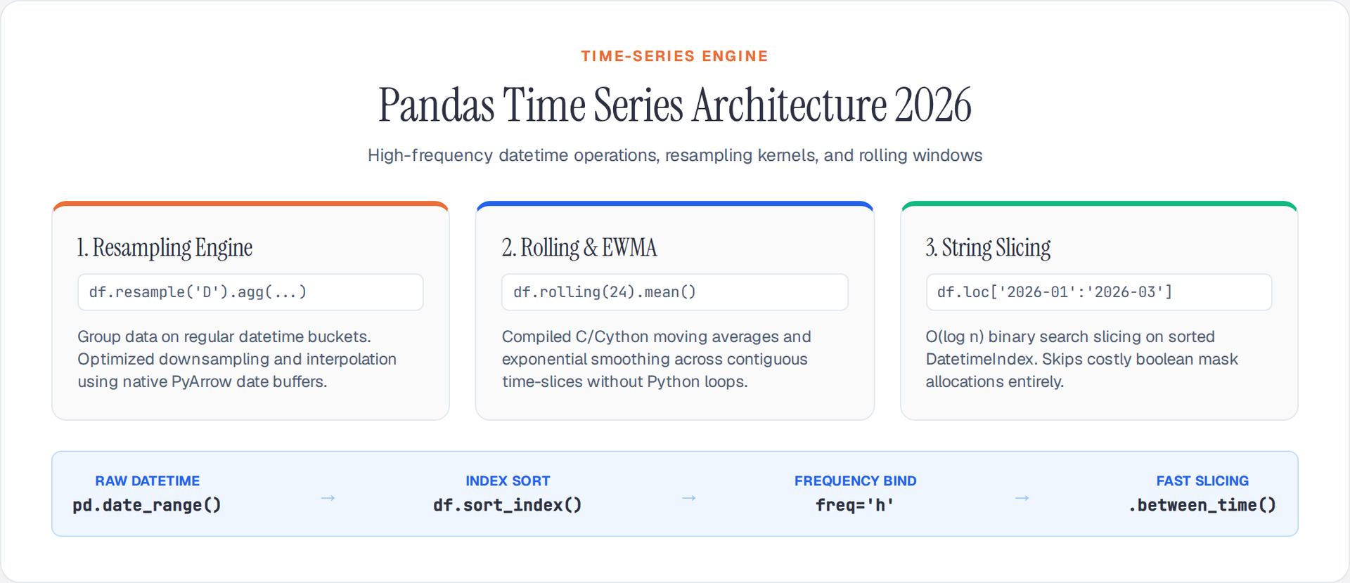
2. High-Performance Resampling

The .resample() method changes time-series frequency (e.g., tick data to daily aggregates). For PyArrow-backed DataFrames, resampling is effectively a fast groupby on datetime boundaries:

# Downsampling: High freq -> Low freq (Aggregating)
# Resample to Daily ('D') frequency and compute mean/sum
daily_summary = df.resample('D').agg({
    'value': ['mean', 'max', 'min']
})

# Resample to End of Business Month ('BME')
monthly_biz = df.resample('BME').sum()

# Upsampling: Low freq -> High freq (Interpolating/Filling)
# Resample Daily to Hourly ('h') and forward-fill missing hours
upsampled_df = daily_summary.resample('h').ffill()

Memory benefit: .resample() partitions data on contiguous datetime blocks. When aggregating float64[pyarrow] numeric columns, it avoids allocating intermediate Python floats.

3. Shifting, Lagging, and Differences

Shifting data generates lagged features — critical for time-series modeling and percentage change metrics:

# Create lagging features for time-series forecasting
df['lag_1h'] = df['value'].shift(periods=1)
df['lag_24h'] = df['value'].shift(periods=24)

# Native period percentage change — optimized C routine
df['pct_change_1h'] = df['value'].pct_change(periods=1)

# Absolute difference — optimized C routine
df['abs_diff'] = df['value'].diff(periods=1)

Key detail: Shifting moves values across the index without modifying index labels. It introduces PyArrow nulls (<NA>) and relies on dtype_backend="pyarrow" to avoid silent conversion to float64 for NaN storage.

4. Rolling and Expanding Windows

Rolling operations compute moving aggregates (e.g., moving averages). Expanding operations compute cumulative metrics (YTD sum).

# Rolling window: Moving 24-hour average
# min_periods=1 allows calculation before full window completes
df['moving_avg_24h'] = df['value'].rolling(window=24, min_periods=1).mean()

# Exponentially Weighted Moving Average (EWMA)
# Faster and smoother than standard SMA
df['ewma_value'] = df['value'].ewm(span=24, adjust=False).mean()

# Expanding window: Cumulative maximum since beginning
df['cumulative_max'] = df['value'].expanding().max()

Pandas 2.x feature: Rolling window calculations dispatch to compiled Cython functions or SciPy operations. Ensure your input columns use native Arrow numerics (Int64[pyarrow], float64[pyarrow]) to bypass Python object boxing overhead during the rolling iteration.

5. Time-Based Slicing and Partial String Indexing

When a DatetimeIndex is sorted, .loc[] supports "partial string indexing", allowing highly expressive and fast time-based subset queries:

# O(log n) slicing via partial string indexing
# Select all data from January 2026
jan_data = df.loc['2026-01']

# Select specific date range
q1_data = df.loc['2026-01-01':'2026-03-31']

# Select all data for a specific day's morning
morning_data = df.loc['2026-05-15 06:00':'2026-05-15 12:00']

# .between_time(): Filter by time-of-day regardless of date
business_hours = df.between_time('09:00', '17:00')

Why it's powerful: Partial string indexing on a sorted DatetimeIndex uses fast binary searching. It avoids creating a boolean mask array (like df[df['date'].dt.month == 1]), making subsetting practically instantaneous on millions of rows.

6. Production Time-Series Patterns

1. Always set and SORT your DatetimeIndex: Unsorted time-indexes lose O(log n) slicing performance and can cause silent errors on .resample().
2. Use specific frequencies: Set df.index.freq = 'h' when possible. Known frequencies unlock rapid datetime math shortcuts.
3. Prefer .between_time() and .at_time(): Use these built-ins instead of boolean masking df.index.hour.
4. Use pyarrow dtype backends: Time-series calculations generate missing values (from shifts and resamples). PyArrow null-bitmaps prevent integer columns from silently upcasting to floats.
5. Leverage exact partial string indexing: df.loc['2026'] is vastly faster than df[df.index.year == 2026].

By combining DatetimeIndex string slicing with compiled .rolling() and .resample() engines, Pandas 2.x remains the benchmark framework for processing high-frequency time-series datasets.